Example 2: Fragmentation¶

In this example, we are going to retrieve MS/MS data from an MGF file and compare it to identification info we read from a pepXML file. We are going to compare the MS/MS spectrum in the file with the theoretical spectrum of a peptide assigned to this spectrum by the search engine.

The script source can be downloaded here. We will also need the example MGF file and the example pepXML file, but the script will download them for you.

The MGF file has a single MS/MS spectrum in it. This spectrum is taken from the SwedCAD database of annotated MS/MS spectra. The pepXML file was obtained by running X!Tandem against the MGF file and converting the results to pepXML with the Tandem2XML tool from TPP.

Let’s start with importing the modules.

from pyteomics import mgf, pepxml, mass, pylab_aux
import os
from urllib.request import urlopen, Request
import pylab

Then we’ll download the files, if needed. Run this if you’re following along on your local machine. Otherwise, just skip this part and suppose we have example.mgf and example.pep.xml in the working directory.

for fname in ('mgf', 'pep.xml'):
    if not os.path.isfile('example.' + fname):
        headers = {'User-Agent': 'Mozilla/5.0 (X11; Linux x86_64) AppleWebKit/537.11 (KHTML, like Gecko) Chrome/23.0.1271.64 Safari/537.11'}
        url = 'http://pyteomics.readthedocs.io/en/latest/_static/example.' + fname
        request = Request(url, None, headers)
        target_name = 'example.' + fname
        with urlopen(request) as response, open(target_name, 'wb') as fout:
            print('Downloading ' + target_name + '...')
            fout.write(response.read())

We’re all set! First of all, let’s read the single spectrum and the corresponding PSM from the files.

with mgf.read('example.mgf') as spectra, pepxml.read('example.pep.xml') as psms:
    spectrum = next(spectra)
    psm = next(psms)

Suppose we just want to visualize the spectrum from MGF. That’s easy!

pylab.figure()
pylab_aux.plot_spectrum(spectrum, title="Experimental spectrum " + spectrum['params']['title'])

At this point, a figure will be created, looking like this:

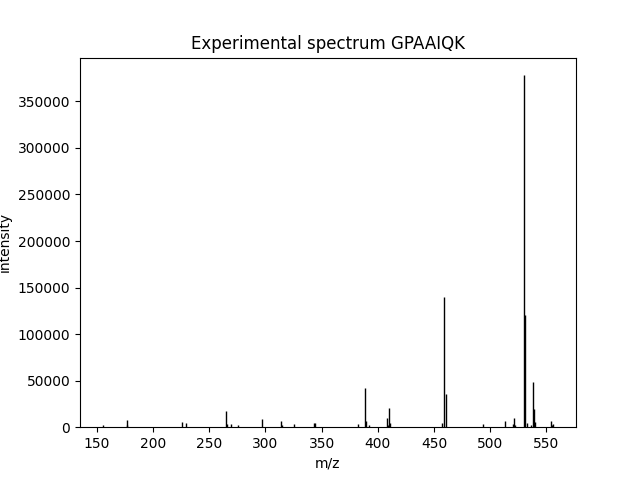
You may not see the figure until you call pylab.show() in the end, depending on your environment.

What if we want to see which peaks actually match the assigned peptide? That is what we call spectrum annotation and it is also easily done:

pylab.figure()
pylab_aux.annotate_spectrum(spectrum, psm['search_hit'][0]['peptide'],
    title='Annotated spectrum ' + psm['search_hit'][0]['peptide'],
    maxcharge=psm['assumed_charge'])

Here’s what you get:

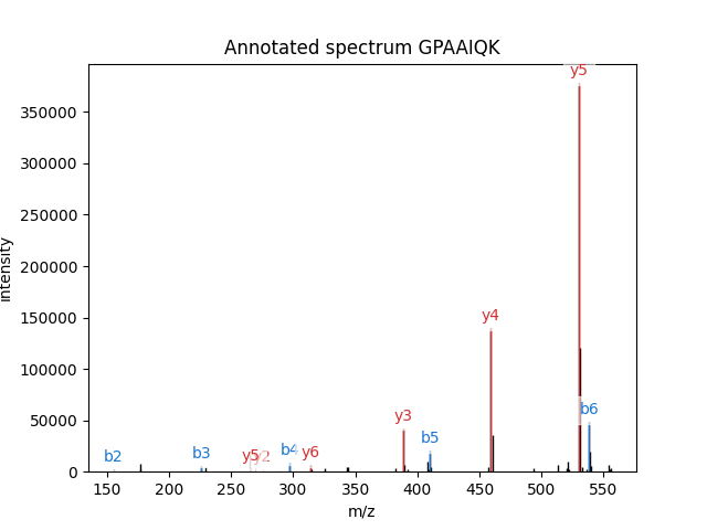
As you can see, pylab_aux.annotate_spectrum() needs a spectrum and a peptide sequence. Check example 4 for more info about spectrum annotation.

Now, suppose we want something else: see all theoretical and observed peaks. There is no readily available function for this, so we’ll have to implement calculation of fragment masses. We will use pyteomics.mass.fast_mass():

def fragments(peptide, types=('b', 'y'), maxcharge=1):
    """
    The function generates all possible m/z for fragments of types
    `types` and of charges from 1 to `maxharge`.
    """
    for i in range(1, len(peptide)):
        for ion_type in types:
            for charge in range(1, maxcharge+1):
                if ion_type[0] in 'abc':
                    yield mass.fast_mass(
                            peptide[:i], ion_type=ion_type, charge=charge)
                else:
                    yield mass.fast_mass(
                            peptide[i:], ion_type=ion_type, charge=charge)

So, the outer loop is over “fragmentation sites”, the next one is over ion types, then over charges, and lastly over two parts of the sequence (C- and N-terminal).

We will use the same function pylab_aux.plot_spectrum() to plot both experimental and theoretical peaks in the same figure. For this, we need to mock a theoretical “spectrum” in the format that the function expects, which is a dictionary with two most important keys, “m/z array” and “intensity array”. We don’t have predicted intensities, so we’ll use the maximum intensity from the experimental spectrum:

fragment_list = list(fragments(psm['search_hit'][0]['peptide'], maxcharge=psm['assumed_charge']))
theor_spectrum = {'m/z array': fragment_list, 'intensity array': [spectrum['intensity array'].max()] * len(fragment_list)}

The rest is easy. Plot two spectra (and tweak them so they’re two different colors), then call pylab.show() to see all figures:

pylab.figure()
pylab.title('Theoretical and experimental spectra for ' + psm['search_hit'][0]['peptide'])
pylab_aux.plot_spectrum(spectrum, width=0.1, linewidth=2, edgecolor='black')
pylab_aux.plot_spectrum(theor_spectrum, width=0.1, edgecolor='red', alpha=0.7)
pylab.show()

The final figure will look like this:

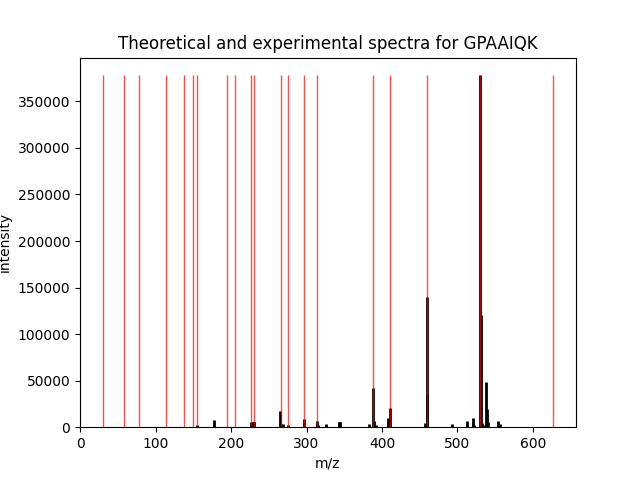
That’s it, as you can see, the most intensive peaks in the spectrum are indeed matched by the theoretical spectrum.